analysis of variance
How much of the variation does each factor explain? Designed experiments rarely vary one thing at a time: a field trial crosses fertilizers with crop varieties, a metabolomics study crosses treatments with genotypes, and samples are run in batches on different days. Analysis of variance splits the spread in a set of measurements into a part explained by each factor and a part left over, the noise, then asks whether each factor explains more than noise alone would, what share of the variation it explains, and whether two factors simply add up or depend on each other. This chapter treats ANOVA as a question asked of a fitted linear model: one factor, its rank-based counterpart, reading the ANOVA table, checking the model, and then two factors and their interaction.
One-page summary (PDF) Jump to the chapter summary
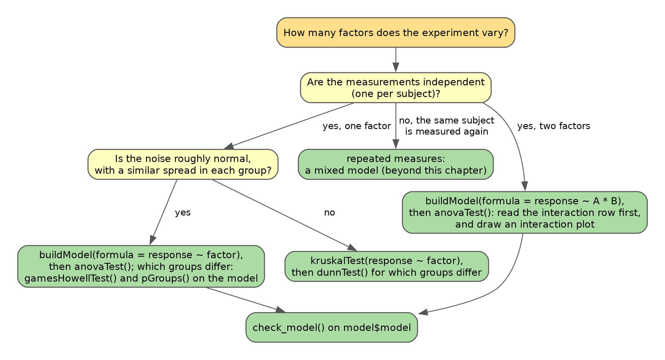
Choosing an analysis of variance. This decision flowchart starts from the number of factors in the experiment and ends at the function to run and the row of the table to read first. Yellow boxes are questions about the design and the data and green boxes are recommended steps.
ANOVA is a linear model
The comparing groups chapter asked whether groups differ, and which pairs. ANOVA asks a broader question: of all the variation in a set of measurements, how much is explained by each factor in the experiment, and how do those factors combine?
The central idea of ANOVA is that the spread in a set of measurements can be split into parts. Spread here means a sum of squares: each measurement’s distance from the grand mean (the average of every measurement), squared, and added up. Some of the spread lies between groups: the group averages sit away from the grand mean. The rest lies within groups: each measurement scatters around its own group’s average. That leftover spread is the noise, the variation the groups do not explain. If the groups truly do not differ, the between-group part should be about the size the noise alone would produce. The F statistic compares the two, each divided by its number of free values (explained below), and a large F means the groups differ by more than noise would allow.
The instrument below builds that split one row at a time, on 30 plants of three species. Press the numbered buttons in order: each draws the distances its row adds up, then fills in the row of the table. The columns are the ones anovaTest() prints, and the next sections explain each of them.
This is the same machinery as the regression chapter, where the r-squared was the share of the total sum of squares a model explains. An ANOVA is a linear model whose predictors are categories rather than numbers (a categorical predictor in an ANOVA is usually called a factor). The formula is written the same way: the response on the left of the ~, the predictors on the right. That connection is what lets ANOVA grow beyond a single factor: anything a linear model can include (a second factor, an interaction, a numeric predictor) can appear in an ANOVA too. It also means the work can be organized the same way throughout this chapter: build the model once with buildModel() and a formula, as in the regression chapter’s section on comparing slopes between groups, then ask that one model questions with anovaTest() and, for a single factor, gamesHowellTest().
concept check
The same 30 plants are in fertilizer_trial. Fill in the blank with the factor the instrument grouped the plants by, then press Run and compare the table with the instrument’s.
Self-check: an ANOVA on potassium in ten aquifers gives a large F. What does that say?
one factor
Using the potassium data from the comparing groups chapter, we build a model of abundance by aquifer, and a one-way ANOVA on it asks whether the aquifers differ at all:
K_model <- buildModel(
  data = K_data,
  model_type = "linear_regression",
  formula = abundance ~ aquifer_code
)

K_model %>%
  anovaTest()
##           term sum_of_squares free_values variance    F
## 1 aquifer_code          150.4           9   16.710 9.49
## 2        noise          169.2          96    1.762   NA
## 3        total          319.6         105       NA   NA
##          p share
## 1 3.28e-10 0.471
## 2       NA 0.529
## 3       NA 1.000
A pretty small p-value! Under the null hypothesis that all aquifers have the same mean, observing differences at least this extreme would be very unlikely, so we have evidence that at least one mean differs. The share column says how much: aquifer explains about 47% of the variation in potassium, and the remaining 53% is noise. The next section reads the rest of the table.
The ANOVA does not say which aquifers differ. That is the job of the Games-Howell test from the comparing groups chapter, which accepts the same model and returns the same letters as gamesHowellTest(abundance ~ aquifer_code) on the data:
K_model %>%
  gamesHowellTest() %>%
  pGroups()
##             treatment  group spaced_group estimate
## aquifer_1   aquifer_1  abcde       abcde  2.325000
## aquifer_10 aquifer_10 abcdef       abcdef 2.328571
## aquifer_2   aquifer_2     af       a    f 3.766667
## aquifer_3   aquifer_3     bd        b d   2.700000
## aquifer_4   aquifer_4      c         c    1.170588
## aquifer_5   aquifer_5     ce         c e  1.450000
## aquifer_6   aquifer_6    abf       ab   f 4.308333
## aquifer_7   aquifer_7      f            f 5.022222
## aquifer_8   aquifer_8  abcde       abcde  2.200000
## aquifer_9   aquifer_9     de          de  1.975758
##               std_err
## aquifer_1  0.43469338
## aquifer_10 0.76180059
## aquifer_2  0.10219806
## aquifer_3  0.15275252
## aquifer_4  0.06228770
## aquifer_5  0.06454972
## aquifer_6  0.57412098
## aquifer_7  0.52566830
## aquifer_8  0.25166115
## aquifer_9  0.22717927
Each aquifer gets its letters, its mean (estimate) and the standard error of that mean (std_err). The standard errors differ a great deal from aquifer to aquifer, because the Games-Howell test uses each group’s own spread rather than the noise variance, the single pooled estimate of the leftover spread that the ANOVA uses. Aquifers 4 and 5, whose wells agree closely, have small standard errors and are told apart from several others, while aquifer 10, whose seven wells scatter widely, shares a letter with every other aquifer.
What the ANOVA adds is a single answer to “is there any difference at all?” and the share of the variation the factor explains. The ANOVA and the Games-Howell test can disagree. An ANOVA can be significant while no single pair is, for example when two groups together sit above a third but neither does on its own, and a Games-Howell test can occasionally flag a pair when the overall ANOVA is not significant. They are answering different questions.
reading the ANOVA table
Each row of an ANOVA table is one term in the model, followed by a row for the noise and a row for the total. Reading across a row:
-
sum_of_squaresis the spread the row accounts for. The rows above the total add up to the total. -
free_valuesis the row’s degrees of freedom, explained below. -
varianceis the sum of squares divided by the free values: the spread per free value. -
Fis the row’s variance divided by the noise variance. -
pis how often noise alone would give an F this large. -
shareis the row’s sum of squares as a share of the total: the share of the variation explained. Every row’s share except the total’s adds up to 1, and the noise row’s share is the part left unexplained.
Free values are what is left once the values the model fixes are spoken for. Each measurement starts out free to take any value. The total row is measured from the grand mean, and once the grand mean is fixed, one measurement is spoken for: knowing the grand mean and all the other measurements pins down the last one. So the 106 potassium measurements leave 105 free values. A factor works the same way on its group means. The ten aquifer means must average out to the grand mean, so once nine of them are known, the tenth is spoken for, which leaves 10 − 1 = 9 free. The noise gets whatever is left: 105 − 9 = 96. Each kind of row has a fixed rule:
| Row of the table | Free values |
|---|---|
| total | the number of measurements − 1 (the grand mean speaks for one) |
| a factor with k groups | k − 1 (the grand mean speaks for one group mean) |
| a numeric predictor | 1 (one slope) |
| an interaction between two terms | the free values of the two terms multiplied together |
| noise | whatever is left: the total’s free values minus every other row’s |
Free values matter because every value a term is free to set lets the model bend toward the data a little, so even a factor with no real effect picks up some spread by chance: on average, about as much per free value as the noise holds. Dividing by free values turns each spread into a variance, and F compares a row’s variance with the noise variance. Aquifer accounts for 150.4 units of spread over 9 free values, a variance of 16.7; the noise holds 169.2 over 96, a variance of 1.76; so F = 16.7 / 1.76 = 9.5. A term with no real effect gives an F near 1 however many free values it has, which is what lets terms of different sizes be compared on the same scale. The noise’s free values matter too: the more there are, the better the noise variance is estimated, and the more the F can be trusted.
Because F is a ratio per free value, it is evidence that a term matters, not a measure of how much it matters: a factor with many groups can explain a great deal of variation and still have a modest F. How much it matters is the share column. Aquifer accounts for 150.4 of the 319.6 units of total spread, a share of 0.47, so aquifer explains about 47% of the variation in potassium and 53% is noise. With a single factor, the share is exactly the r-squared from the regression chapter.
concept check
Fill in the blank so the table works out the noise’s free values from the rules above, then press Run and compare the result with the free_values column of the ANOVA table.
Self-check: a trial compares four fertilizers with six plots each. How many free values do the fertilizer row and the noise row have?
the Kruskal test
The rank-based cousin of the ANOVA is the Kruskal test. It is the Wilcox test extended to more than two groups: it pools every value from every group, ranks them all together, and asks whether the groups’ average ranks differ by more than chance would allow. It behaves much like an ANOVA run on the ranks, which is why it does not need normally distributed data. It answers only the “any difference at all?” question for a single factor, and which groups differ is then a question for the Dunn test from the comparing groups chapter. Rank-based versions of the designs in the rest of this chapter do exist, but they are more specialized and are not covered here.
K_data %>%
  kruskalTest(abundance ~ aquifer_code)
## # A tibble: 1 × 6
##   .y.           n statistic    df             p method
## * <chr>     <int>     <dbl> <int>         <dbl> <chr>
## 1 abundance 106 55.9 9 0.00000000807 Kruskal-Wal…checking the model
An ANOVA makes the same assumptions as the linear models in the regression chapter, and they are all assumptions about the noise: each measurement’s distance from its group mean (which check_model() calls a residual) should be roughly normal and have a similar spread in every group, and the measurements should be independent. The check_model() habit from the regression chapter applies here unchanged:
check_model(K_model$model)
Diagnostic checks for the one-way ANOVA model of potassium by aquifer. Panels produced by check_model(): a posterior predictive check comparing the distribution of observed and model-predicted potassium; linearity and homogeneity of variance, each plotting residuals against fitted values (one vertical stripe per aquifer); influential observations, plotting standardized residuals against leverage; and normality of residuals as a quantile-quantile plot. Data are from the hawaii_aquifers dataset.
Unequal spreads matter most to the ANOVA’s F, which compares every term with one noise variance pooled across all the groups. The Games-Howell test used above to find which groups differ already judges each pair on its own two spreads, so it does not depend on this assumption. When the spreads clearly differ between groups, a Welch ANOVA is the unequal-variance counterpart of the ANOVA, and the rank-based Kruskal test is another way out for a single factor.
two factors and interactions
Many experiments vary more than one thing at once: a treatment and a genotype, a fertilizer and a soil type, an analyte and a site. A two-way ANOVA splits the spread into a part for each factor, a part for their interaction, and the noise, and asks whether the two interact, meaning whether the effect of one factor depends on the level of the other.
The instrument below adds a second factor to the 30 plants: half of each species was given fertilizer. After the species row, the fertilizer row draws how far each fertilizer mean sits from the grand mean. The interaction row then asks where each species-and-fertilizer combination would sit if fertilizer did the same for every species (the dashed lines), and draws how far each real combination sits from there. The noise is now each plant’s distance from its own combination’s mean, and it is far smaller than in the one-factor table, because the fertilizer and interaction rows now explain spread that used to count as noise.
As an example in real data, consider sodium and chloride in four of the aquifers:
nacl <- hawaii_aquifers %>%
  filter(analyte %in% c("Na", "Cl"),
         aquifer_code %in% c("aquifer_1", "aquifer_2", "aquifer_3", "aquifer_4"))

nacl_model <- buildModel(
  data = nacl,
  model_type = "linear_regression",
  formula = abundance ~ analyte * aquifer_code
)

nacl_model %>%
  anovaTest()
##                   term sum_of_squares free_values variance
## 1              analyte           7031           1   7031.0
## 2         aquifer_code          22050           3   7349.0
## 3 analyte:aquifer_code           3845           3   1282.0
## 4                noise          32940          68    484.4
## 5                total          65860          75       NA
##       F        p share
## 1 14.51 3.02e-04 0.107
## 2 15.17 1.17e-07 0.335
## 3  2.65 5.60e-02 0.058
## 4    NA       NA 0.500
## 5    NA       NA 1.000
The * in the formula asks for both factors and their interaction. The table has one row for each, then the noise and the total, and the free values still follow the rules: the 76 measurements leave 75 once the grand mean is spoken for, analyte (two levels) takes 1, aquifer (four levels) takes 3, the interaction takes 1 × 3 = 3, and the noise keeps the remaining 68. Analyte explains about 11% of the variation (chloride is more abundant than sodium overall) and aquifer about 33%. The interaction row asks whether the gap between chloride and sodium is the same in every aquifer. It explains about 6% of the variation, and its p-value is 0.056, just above the usual threshold, so the evidence that the gap changes from aquifer to aquifer is suggestive but not conclusive. An interaction plot shows what the row is testing: one line per analyte across the aquifers. Parallel lines mean no interaction; lines that converge, diverge or cross mean the effect of one factor depends on the other.
nacl %>%
  group_by(aquifer_code, analyte) %>%
  summarize(mean_abundance = mean(abundance)) %>%
  ggplot(aes(x = aquifer_code, y = mean_abundance, color = analyte, group = analyte)) +
    geom_point(size = 3) +
    geom_line() +
    theme_bw()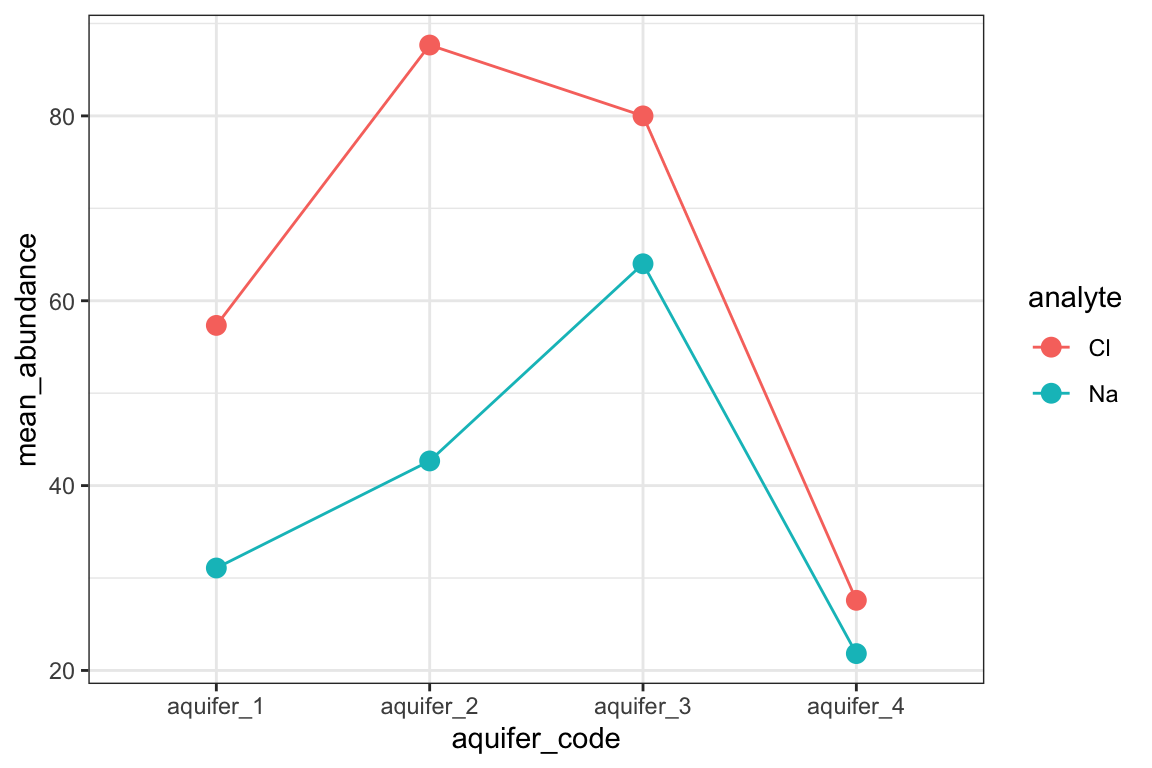
Chloride and sodium in four Hawaiian aquifers. Interaction plot of mean abundance (y axis) for each aquifer (x axis), with one line and color per analyte; each point is the mean of all wells sampled in that aquifer. The gap between chloride and sodium is wide in aquifer 2 and narrow in aquifer 4, which is what the interaction term in the two-way ANOVA tests. Data are from the hawaii_aquifers dataset.
The interaction row is not “the two factors together”. It holds only the extra spread explained by letting the effect of one factor differ across the levels of the other, on top of what the two factors explain on their own. Most of the explaining is usually done by the factors themselves, so the interaction row often has the smallest share, and that is expected. When an interaction is real, though, the main effects on their own can mislead: “the treatment raises yield” is not a useful summary if it raises yield in one soil and lowers it in another. Read the interaction row first.
other designs
The same model-then-table approach covers several designs that come up in laboratory work. They are named here so they can be recognized; each has its own literature.
-
Blocking. Samples run on different days, plates or instrument batches can shift by batch alone. A block is a factor that is not of interest but adds variation; including it, as in
response ~ treatment + batch, moves that variation out of the noise and makes the factor of interest easier to detect. -
Adjusting for a covariate (ANCOVA). When groups also differ in a numeric variable that affects the response, such as plant size, adding it to the formula,
response ~ treatment + plant_size, compares the groups at the same value of the covariate. With*instead of+, the model gives each group its own slope, which is the comparing-slopes analysis from the regression chapter. - Repeated measures. When the same subject is measured more than once (the same plant over several weeks, the same patient before and after a treatment), the measurements are not independent, and treating them as if they were overstates the evidence. These designs need a mixed model, which tracks which measurements belong to which subject.
- Many responses at once. MANOVA extends ANOVA to several responses measured on each sample but assumes they are jointly normal, which large chemical profiles rarely are. PERMANOVA works from a distance matrix, as built in the distances and scaling chapter, and gets its p-value by shuffling the group labels, so it is the usual choice for metabolomics and community profiles.
practice

chapter summary
Download this summary as a one-page PDF
An ANOVA splits the spread in a response (its sum of squares) into the part each term explains and the part left over, the noise. Build the model, then ask it questions: fit it once with a formula (response on the left, factors on the right, * for an interaction), read the ANOVA table, then, for a single factor, use the Games-Howell test on the same model to find which groups differ. Read the table row by row: each row’s free values are what is left once the values the model fixes are spoken for (the grand mean speaks for one measurement, a factor with k groups keeps k − 1, an interaction multiplies its terms’, and the noise gets the rest). A row’s variance is its sum of squares per free value, F is that variance over the noise variance, so it is evidence that a term matters, and share is how much: the row’s share of the variation explained, with every row’s share adding up to 1. With two factors, read the interaction row first: if it is real, a main effect alone can mislead, and an interaction plot shows how. Check the model before trusting it: noise roughly normal with a similar spread in every group, and measurements independent (repeated measurements of one subject need a mixed model). For a single factor with non-normal data, use the Kruskal test, then the Dunn test.
| Function | What it is for | How it is used in this chapter |
|---|---|---|
buildModel(formula = ) |
fitting the model the ANOVA is read from |
response ~ factor, or response ~ factor_1 * factor_2 for an interaction, with model_type = "linear_regression"
|
anovaTest() |
the ANOVA table: a row per term, then noise and total, with sum_of_squares, free_values, variance, F, p and share
|
piped after the model |
gamesHowellTest(), pGroups()
|
which groups differ, as letters, using each group’s own spread | piped after the same one-factor model |
kruskalTest(abundance ~ aquifer_code) |
rank-based test of any difference, one factor | on the data, followed by dunnTest()
|
check_model() |
diagnostic panels for the noise (residuals) | given model$model
|
further reading
Common statistical tests are linear models. Jonas Lindeløv shows that the t-test, one- and two-way ANOVA and ANCOVA are all the same linear model with different predictors, with R code side by side. It is the clearest account of the idea this chapter is built on.
Analysis of variance and blocking. Martin Krzywinski and Naomi Altman’s short Nature Methods column (2014) explains the between- and within-group split behind F, and how a blocking factor removes nuisance variation from the error term.
Two-way anova. John McDonald’s Handbook of Biological Statistics walks through two-way designs with and without replication, what an interaction test does, and why main effects can mislead when an interaction is present.
Interaction analysis in emmeans. The vignette for the package the course uses to compare slopes between groups shows how to follow up an interaction: comparisons within each level of the other factor, interaction plots, and comparing slopes between groups.