installation

R
R is the computing language we will use to run our analyses and produce high quality plots. If you already have R installed (you will need at least version 4.1.1), you can go straight to installing RStudio. If not, follow these steps to install R:
Click on “Download R for <your operating system>” (see footnote), depending on your operating system you will select “Download R for Linux”, “Download R for (Mac) OS X”, or “Download R for Windows”.
We will use <this notation> quite a bit. It indicates a place where you should insert information, data, or something similar that corresponds to your particular situation. In this example it means insert “your operating system”, i.e. Linux, (Mac) OS X, or Windows.
For Mac: download the .pkg file for the latest release. For PC: click “install R for the first time”, then click “Download R <version> for Windows”.
After the executable finishes downloading (in Windows, it is a file with .exe extension; for Mac, it is a .dmg file or a .dmg inside a .pkg file), open the file as an administrator, and follow the installation instructions. R should install without any problems. You can click OK for all of the windows that pop-up during installation, and choose a “regular” installation (if given the choice).
If you have trouble installing R please google “Install R Mac” or “Install R PC” and follow one the many video tutorials out there. If you have tried this and are still having trouble, please contact me.
RStudio
Once we install R, we can install RStudio, which is essentially a convenient way of interacting with R. Some people do not like RStudio and prefer to interact with R directly. This is fine, but many beginning R users find RStudio helpful, so I recommend it. Follow these steps to install RStudio:
Go to https://rstudio.com/
Click “DOWNLOAD” at the top of the page.
Click the “DOWNLOAD” button that corresponds to RStudio Desktop with the free Open Source License.
The page may automatically detect which operating system you are using and recommend a version for you. If it does, download that file (.exe for PC or .dmg for Mac). If not, scroll down to the “All Installers” section and download the file that is right for you. Open the file as an administrator, and follow the installation instructions. RStudio should install without any problems. You can click OK for all of the windows that pop-up during installation, and choose a “regular” installation (if given the choice).
If you have trouble installing RStudio please google “Install RStudio Mac” or “Install RStudio PC” and following one the many video tutorials out there. If you have tried this and are still having trouble, please contact me.
verification
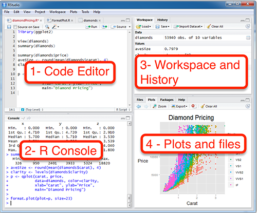
Open RStudio by clicking on the appropriate file in your applications folder, or wherever it is saved on your computer. If you are on Windows, be sure to run RStudio as administrator. You will see several windows. One is the Code Editor, one is the R Console, one is the Workspace and History, and one is the Plots and Files window.
The R Console window should have a > in it. Type head(Indometh). This should display the first six lines of a data set describing the pharmacokinets of indomethacin. This is one of the built in datasets in R - you do not need any additional files to run this test.
head(Indometh)
## Grouped Data: conc ~ time | Subject
##   Subject time conc
## 1       1 0.25 1.50
## 2       1 0.50 0.94
## 3       1 0.75 0.78
## 4       1 1.00 0.48
## 5       1 1.25 0.37
## 6       1 2.00 0.19
Next, type plot(Indometh) into the R Console. This will plot the indomethacin dataset in a basic way.
plot(Indometh)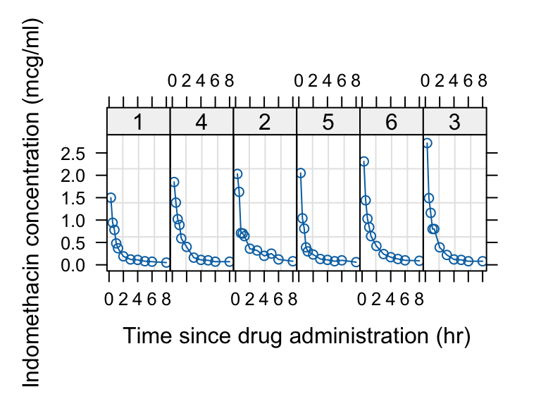
If both the above commands (head(Indometh) and plot(Indometh)) worked and there were no error messages during installation, then you should be ready to proceed.
TeX
In this class we will generate high quality reports suitable for submission to supervisors, academic journals, etc. For this, we need the typesetting engine TeX. There are a few ways to do this. The easiest way is using the following commands:
install.packages(c('tinytex', 'rmarkdown'))If you are on Mac, you may get an error about “not being able to write to a path” or something like that. In that case you probably need to open your terminal and run the following two commands:
sudo chown -R \`whoami\`:admin /usr/local/binand then
~/Library/TinyTeX/bin/\*/tlmgr path addThen, on both Mac and PC, you then need to do:
tinytex::install_tinytex()Other options are: if you have Windows, download and install MikTeX. If you have OSX, you can download and install MacTeX.
phylochemistry
In addition to the tidyverse, there are a variety of other packages we will need, as well as some datasets and custom functions. These call all be loaded by doing the following.
First, attempt to load phylochemistry, if you are on Windows, be sure you’ve opened RStudio as an administrator (right click, “run as administrator”):
source("https://thebustalab.github.io/phylochemistry/phylochemistry.R")The first time you try this, it will very likely say: “You need to install the following packages before proceeding […] Is it okay if phylochemistry installs them for you?” You should say “yes”.
data import
Once R, RStudio, and phylochemistry are installed, the last piece is getting your own data into R. The sandboxes in this book load their datasets for you, but data sitting on your own hard drive has to be imported, and there are two ways to do it.
The easiest way to do this is to use the interactive command readCSV(), a function that comes with the phylochemistry source command. You run readCSV() in your console, then navigate to the data on your hard drive.
Another option is to read the data in from a path. For this, you will need to know the “path” to your data file. This is essentially the street address of your data on your computer’s hard drive. Paths look different on Mac and PC.
- On Mac:
/Users/lucasbusta/Documents/sample_data_set.csv(note the forward slashes!) - On PC:
C:\\My Computer\\Documents\\sample_data_set.csv(note double backward slashes!)
You can quickly find paths to files via the following:
- On Mac: Locate the file in Finder. Right-click on the file, hold the Option key, then click “Copy
as Pathname” - On PC: Locate the file in Windows Explorer. Hold down the Shift key then right-click on the file. Click “Copy As Path”
With these paths, we can read in data using the read_csv command. We’ll run read_csv("<path_to_your_data>"). Note the use of QUOTES ""! Those are necessary. Also make sure your path uses the appropriate direction of slashes for your operating system.