phylogenies

buildTree

This function is a swiss army knife for tree building. It takes as input alignments or existing phylogenies from which to derive a phylogeny of interest, it can use neighbor-joining or maximum liklihood methods (with model optimization), it can run bootstrap replicates, and it can calculate ancestral sequence states. To illustrate, let’s look at some examples:

newick input

Let’s use the Busta lab’s plant phylogeny [derived from Qian et al., 2016] to build a phylogeny with five species in it.

tree <- buildTree(
  scaffold_type = "newick",
  scaffold = "https://thebustalab.github.io/data/plant_phylogeny.newick",
  members = c("Sorghum_bicolor", "Zea_mays", "Setaria_viridis", "Arabidopsis_thaliana", "Amborella_trichopoda")
)
## Pro tip: most tree read/write functions reset node numbers. Fortify your tree and save it as a csv file to preserve node numbering.


tree
## 
## Phylogenetic tree with 5 tips and 4 internal nodes.
## 
## Tip labels:
##   Amborella_trichopoda, Zea_mays, Sorghum_bicolor, Setaria_viridis, Arabidopsis_thaliana
## Node labels:
##   , , , 
## 
## Rooted; includes branch lengths.


plot(tree)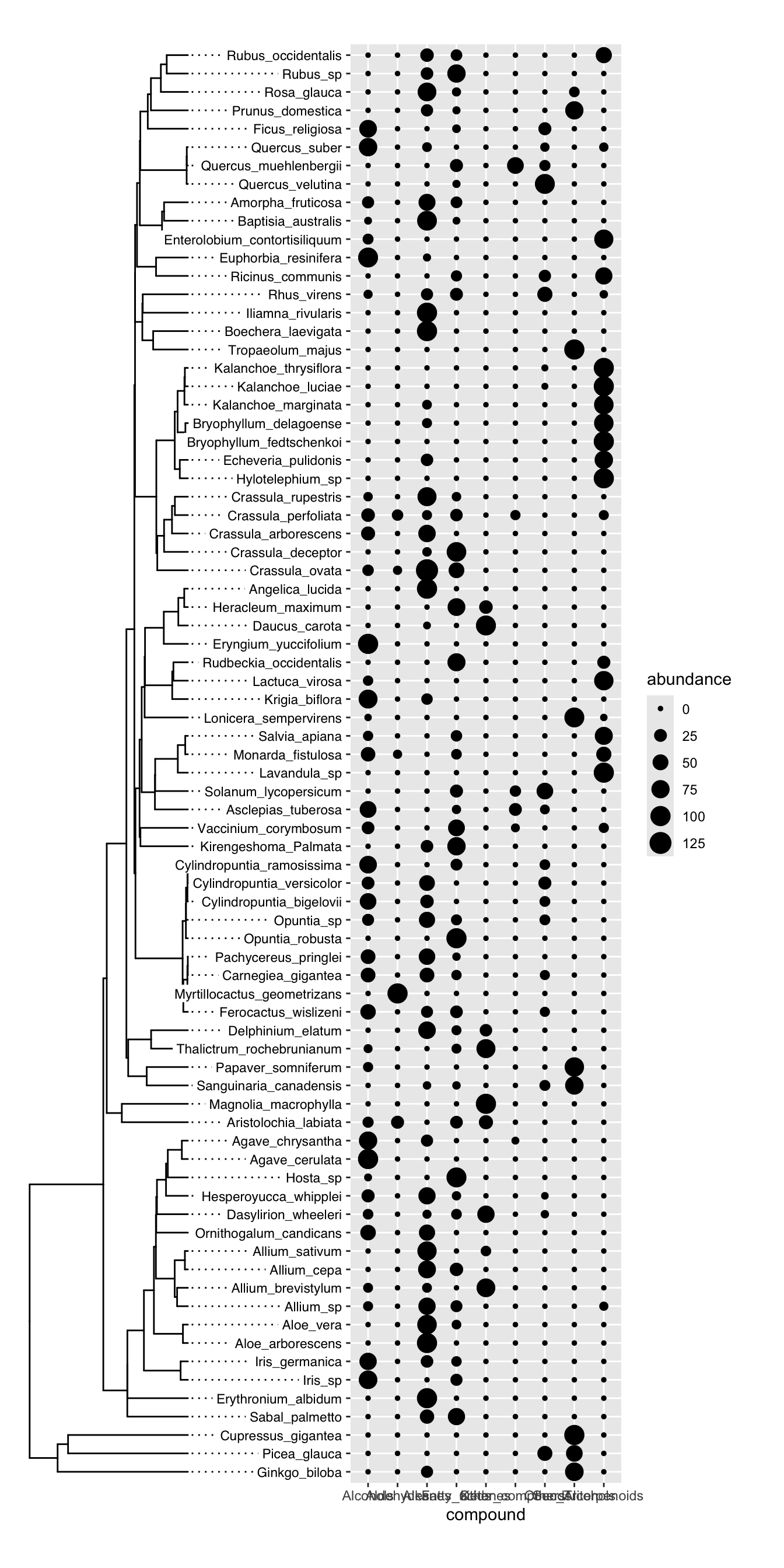

Cool! We got our phylogeny. What happens if we want to build a phylogeny that has a species on it that isn’t in our scaffold? For example, what if we want to build a phylogeny that includes Arabidopsis neglecta? We can include that name in our list of members:

tree <- buildTree(
  scaffold_type = "newick",
  scaffold_in_path = "https://thebustalab.github.io/data/plant_phylogeny.newick",
  members = c("Sorghum_bicolor", "Zea_mays", "Setaria_viridis", "Arabidopsis_neglecta", "Amborella_trichopoda")
)
## IMPORTANT: Some species substitutions or removals were made as part of buildTree. Run build_tree_substitutions() to see them all.
## Pro tip: most tree read/write functions reset node numbers. Fortify your tree and save it as a csv file to preserve node numbering.


tree
## 
## Phylogenetic tree with 5 tips and 4 internal nodes.
## 
## Tip labels:
##   Amborella_trichopoda, Zea_mays, Sorghum_bicolor, Setaria_viridis, Arabidopsis_neglecta
## Node labels:
##   , , , 
## 
## Rooted; includes branch lengths.


plot(tree)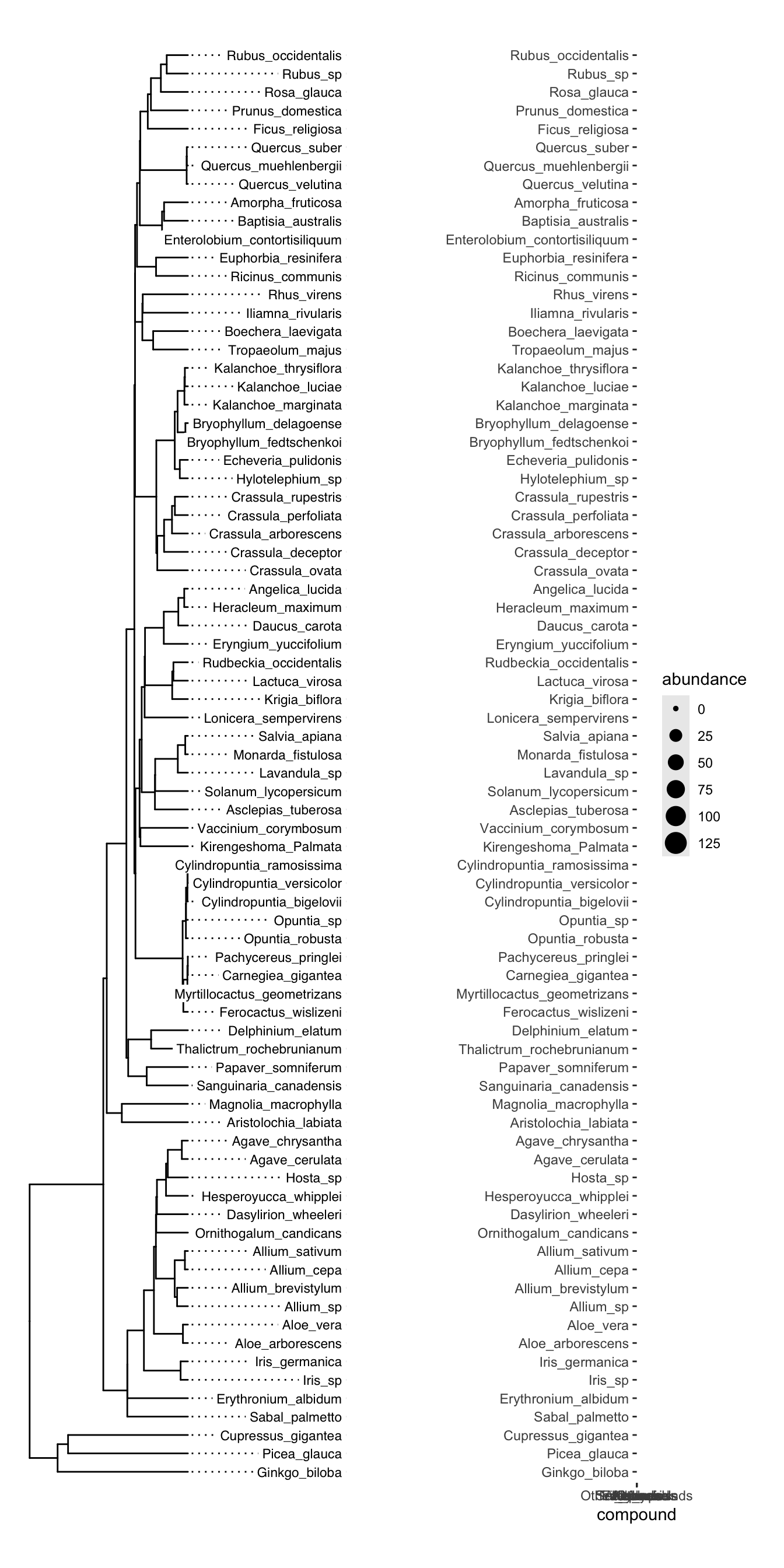

Note that buildTree informs us: “Scaffold newick tip Arabidopsis_thaliana substituted with Arabidopsis_neglecta”. This means that Arabidopsis neglecta was grafted onto the tip originally occupied by Arabidopsis thaliana. This behaviour is useful when operating on a large phylogenetic scale (i.e. where exact phylogeny topology is not critical below the family level). However, if a person is interested in using an existing newick tree as a scaffold for a phylogeny where genus-level topology is critical, then beware! Your scaffold may not be appropriate if you see that message. When operating at the genus level, you probably want to use sequence data to build your phylogeny anyway. So let’s look at how to do that:

alignment input

Arguments in this case are:

“scaffold_type”: “amin_alignment” or “nucl_alignment” for amino acids or nucleotides.
“scaffold_in_path”: path to the fasta file that contains the alignment from which you want to build a tree.
“ml”: Logical, TRUE if you want to use maximum liklihood, FALSE if not, in which case neighbor joining will ne used.
“model_test”: if you say TRUE to “ml”, should buildTree test different maximum liklihood models and then use the “best” one?
“bootstrap”: TRUE or FALSE, whether you want bootstrap values on the nodes.
“ancestral_states”: TRUE or FALSE, should buildTree() compute the ancestral sequence at each node?
“root”: NULL, or the name of an accession that should form the root of the tree.

buildTree(
  scaffold_type = "amin_alignment",
  scaffold_in_path = "/path_to/a_folder_for_alignments/all_amin_seqs.fa",
  ml = FALSE, 
  model_test = FALSE,
  bootstrap = FALSE,
  ancestral_states = FALSE,
  root = NULL
)

plotting trees

There are several approaches to plotting trees. A simple one is using the base plot function:

test_tree_small <- buildTree(
  scaffold_type = "newick",
  scaffold_in_path = "https://thebustalab.github.io/data/plant_phylogeny.newick",
  members = c("Sorghum_bicolor", "Zea_mays", "Setaria_viridis")
)
## Pro tip: most tree read/write functions reset node numbers. Fortify your tree and save it as a csv file to preserve node numbering.


plot(test_tree_small)

Though this can get messy when there are lots of tip labels:

set.seed(122)
test_tree_big <- buildTree(
  scaffold_type = "newick",
  scaffold_in_path = "https://thebustalab.github.io/data/plant_phylogeny.newick",
  members = plant_species$Genus_species[abs(floor(rnorm(60)*100000))]
)

plot(test_tree_big)

One solution is to use ggtree, which by default doesn’t show tip labels. plot can do that too, but ggtree does a bunch of other useful things, so I recommend that:

ggtree(test_tree_big)

Another convenient fucntion is ggplot’s fortify. This will convert your phylo object into a data frame:

test_tree_big_fortified <- fortify(test_tree_big)
test_tree_big_fortified
## # A tbl_tree abstraction: 101 × 9
## # which can be converted to treedata or phylo 
## # via as.treedata or as.phylo
##    parent  node branch.length label isTip     x     y branch
##     <int> <int>         <dbl> <chr> <lgl> <dbl> <dbl>  <dbl>
##  1     54     1          83.0 Wolf… TRUE   188.     1   147.
##  2     54     2          83.0 Spat… TRUE   188.     2   147.
##  3     55     3         138.  Dios… TRUE   188.     3   120.
##  4     58     4          42.7 Bulb… TRUE   188.     5   167.
##  5     58     5          42.7 Ober… TRUE   188.     6   167.
##  6     59     6          32.0 Poma… TRUE   188.     7   172.
##  7     59     7          32.0 Teli… TRUE   188.     8   172.
##  8     56     8         135.  Cala… TRUE   188.     4   121.
##  9     61     9         147.  Pepe… TRUE   188.     9   115.
## 10     62    10         121.  Endl… TRUE   188.    10   128.
## # ℹ 91 more rows
## # ℹ 1 more variable: angle <dbl>

ggtree can still plot this dataframe, and it allows metadata to be stored in a human readable format by using mutating joins (explained below). This metadata can be plotted with standard ggplot geoms, and these dataframes can also conveniently be saved as .csv files:


## Note that "plant_species" comes with the phylochemistry source.

test_tree_big_fortified_w_data <- left_join(test_tree_big_fortified, plant_species, by = c("label" = "Genus_species"))

test_tree_big_fortified_w_data
## # A tbl_tree abstraction: 101 × 14
## # which can be converted to treedata or phylo 
## # via as.treedata or as.phylo
##    parent  node branch.length label isTip     x     y branch
##     <int> <int>         <dbl> <chr> <lgl> <dbl> <dbl>  <dbl>
##  1     54     1          83.0 Wolf… TRUE   188.     1   147.
##  2     54     2          83.0 Spat… TRUE   188.     2   147.
##  3     55     3         138.  Dios… TRUE   188.     3   120.
##  4     58     4          42.7 Bulb… TRUE   188.     5   167.
##  5     58     5          42.7 Ober… TRUE   188.     6   167.
##  6     59     6          32.0 Poma… TRUE   188.     7   172.
##  7     59     7          32.0 Teli… TRUE   188.     8   172.
##  8     56     8         135.  Cala… TRUE   188.     4   121.
##  9     61     9         147.  Pepe… TRUE   188.     9   115.
## 10     62    10         121.  Endl… TRUE   188.    10   128.
## # ℹ 91 more rows
## # ℹ 6 more variables: angle <dbl>, Phylum <chr>,
## #   Order <chr>, Family <chr>, Genus <chr>, species <chr>


ggtree(test_tree_big_fortified_w_data) + 
  geom_point(
    data = filter(test_tree_big_fortified_w_data, isTip == TRUE),
    aes(x = x, y = y, fill = Order), size = 3, shape = 21, color = "black") +
  geom_text(
    data = filter(test_tree_big_fortified_w_data, isTip == TRUE),
    aes(x = x, y = y, label = y), size = 2, color = "white") +
  geom_tiplab(aes(label = label), offset = 10, size = 2) +
  theme_void() +
  scale_fill_manual(values = discrete_palette) +
  coord_cartesian(xlim = c(0,280)) +
  theme(
    legend.position = c(0.15, 0.75)
  )

collapseTree

Sometimes we want to view a tree at a higher level of taxonomical organization, or some other higher level. This can be done easily using the collapseTree function. It takes two arguments: an un-fortified tree (tree), and a two-column data frame (associations). In the first column of the data frame are all the tip labels of the tree, and in the second column are the higher level of organization to which each tip belongs. The function will prune the tree so that only one member of the higher level of organization is included in the output. For example, let’s look at the tree from the previous section at the family level:

collapseTree(
  tree = test_tree_big,
  associations = data.frame(
    tip.label = test_tree_big$tip.label,
    family = plant_species$Family[match(test_tree_big$tip.label, plant_species$Genus_species)]
  )
) -> test_tree_big_families
## Branch lengths have been set to one.


ggtree(test_tree_big_families) + geom_tiplab() + coord_cartesian(xlim = c(0,300))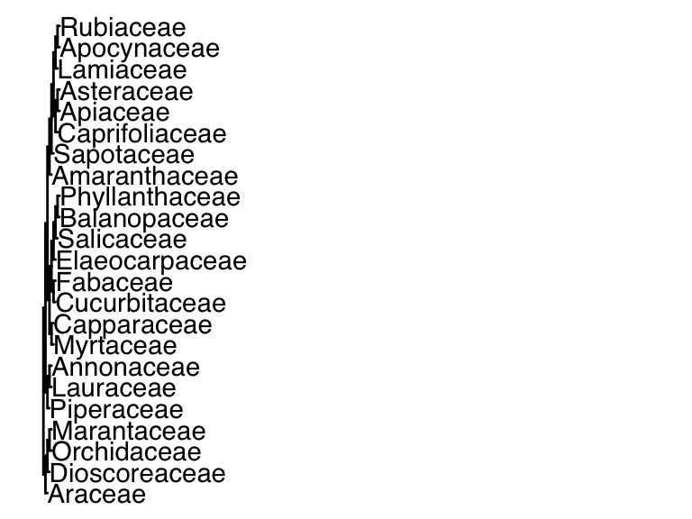

trees and traits

To plot traits alongside a tree, we can use ggtree in combination with ggplot. Here is an example. First, we make the tree:

chemical_bloom_tree <- buildTree(
  scaffold_type = "newick",
  scaffold_in_path = "http://thebustalab.github.io/data/angiosperms.newick",
  members = unique(chemical_blooms$label)
)
## IMPORTANT: Some species substitutions or removals were made as part of buildTree. Run build_tree_substitutions() to see them all.
## Pro tip: most tree read/write functions reset node numbers. Fortify your tree and save it as a csv file to preserve node numbering.

Next we join the tree with the data:

data <- left_join(fortify(chemical_bloom_tree), chemical_blooms)
## Joining with `by = join_by(label)`

head(data)
## # A tibble: 6 × 18
##   parent  node branch.length label  isTip     x     y branch
##    <int> <int>         <dbl> <chr>  <lgl> <dbl> <dbl>  <dbl>
## 1     80     1         290.  Ginkg… TRUE   352.     1   207.
## 2     81     2         267.  Picea… TRUE   352.     2   219.
## 3     81     3         267.  Cupre… TRUE   352.     3   219.
## 4     84     4         135.  Eryth… TRUE   352.     5   285.
## 5     86     5          16.2 Iris_… TRUE   352.     6   344.
## 6     86     6          16.2 Iris_… TRUE   352.     7   344.
## # ℹ 10 more variables: angle <dbl>, Alkanes <dbl>,
## #   Sec_Alcohols <dbl>, Others <dbl>, Fatty_acids <dbl>,
## #   Alcohols <dbl>, Triterpenoids <dbl>, Ketones <dbl>,
## #   Other_compounds <dbl>, Aldehydes <dbl>

Now we can plot the tree:

tree_plot <- ggtree(data) +
  geom_tiplab(
    align = TRUE, hjust = 1, offset = 350,
    geom = "label", label.size = 0, size = 3
  ) +
  scale_x_continuous(limits = c(0,750))

IMPORTANT! When we plot the traits, we need to reorder whatever is on the shared axis (in this case, the y axis) so that it matches the order of the tree. In this case, we need to reorder the species names so that they match the order of the tree. We can do this by using the reorder function, which takes two arguments: the thing to be reordered, and the thing to be reordered by. In this case, we want to reorder the species names by their y coordinate on the tree. We can do this by using the y column of the data frame that we created when we fortified the tree. We can then plot the traits:

trait_plot <- ggplot(
    data = pivot_longer(
      filter(data, isTip == TRUE),
      cols = 10:18, names_to = "compound", values_to = "abundance"
    ),
    aes(x = compound, y = reorder(label, y), size = abundance)
  ) +
  geom_point() +
  scale_y_discrete(name = "") +
  theme(
    plot.margin = unit(c(1,1,1,1), "cm")
  )

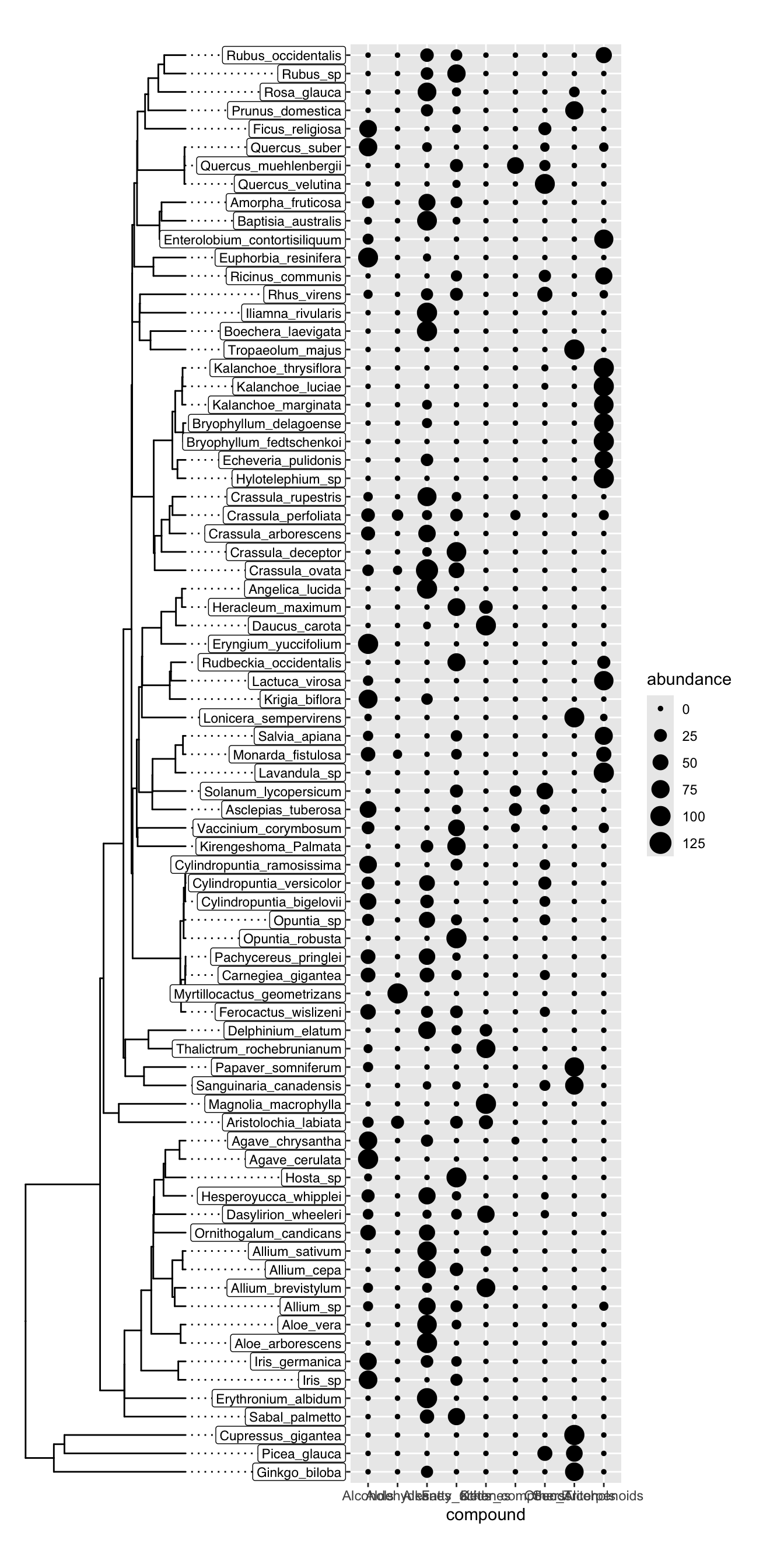
Finally, we can plot the two plots together using plot_grid. It is important to manually inspect the tree tips and the y axis text to make sure that everything lines up. We don’t want to be plotting the abundance of one species on the y axis of another species. In this case, everything looks good:

plot_grid(
  tree_plot,
  trait_plot,
  nrow = 1, align = "h", axis = "tb"
)

Once our manual inspection is complete, we can make a new version of the plot in which the y axis text is removed from the trait plot and we can reduce the margin on the left side of the trait plot to make it look nicer:

tree_plot <- ggtree(data) +
  geom_tiplab(
    align = TRUE, hjust = 1, offset = 350,
    geom = "label", label.size = 0, size = 3
  ) +
  scale_x_continuous(limits = c(0,750))

trait_plot <- ggplot(
    data = pivot_longer(
      filter(data, isTip == TRUE),
      cols = 10:18, names_to = "compound", values_to = "abundance"
    ),
    aes(x = compound, y = reorder(label, y), size = abundance)
  ) +
  geom_point() +
  scale_y_discrete(name = "") +
  theme(
    axis.text.y = element_blank(),
    plot.margin = unit(c(1,1,1,-1.5), "cm")
  )

plot_grid(
  tree_plot,
  trait_plot,
  nrow = 1, align = "h", axis = "tb"
)

alignments

phylogenetic analyses

Integrated Bioanalytics