6 clustering
6.1 theory
“Which of my samples are most closely related?”
So far we have been looking at how to plot raw data, as well as data that has been summarize across samples. This is important stuff and very useful. However, we often have questions about how samples in our datasets relate to one another. For example: in the Alaska lakes dataset, which lake is most similar, chemically speaking, to Lake Narvakrak? Answering this requires calculating numeric distances between samples based on their chemical properties. For this, and other questions, we need to use matrix analyses. For this, we will use runMatrixAnalysis(), a function that is loaded into your R Session when you run the source() command.
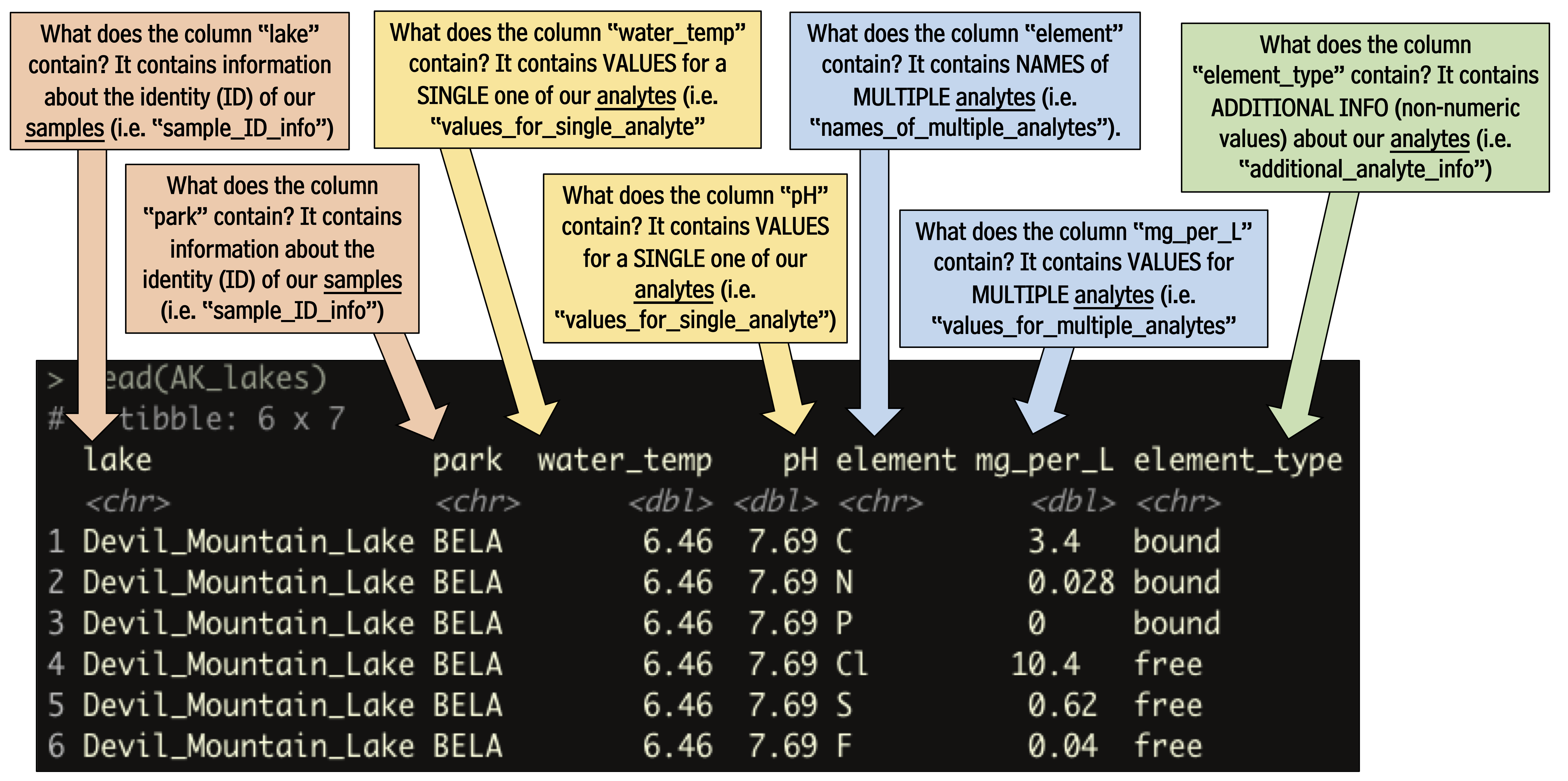
Matrix analyses can be a bit difficult to set up. There are two things that we can do to help us with this: (i) we will use a template for runMatrixAnalysis() (see below) and (ii) it is critical that we think about our data in terms of samples and analytes. Let’s consider our Alaska lakes data set:
alaska_lake_data
## # A tibble: 220 × 7
##    lake                park  water_temp    pH element mg_per_L element_type
##    <chr>               <chr>      <dbl> <dbl> <chr>      <dbl> <chr>
##  1 Devil_Mountain_Lake BELA        6.46  7.69 C          3.4   bound
##  2 Devil_Mountain_Lake BELA        6.46  7.69 N          0.028 bound
##  3 Devil_Mountain_Lake BELA        6.46  7.69 P          0     bound
##  4 Devil_Mountain_Lake BELA        6.46  7.69 Cl        10.4   free
##  5 Devil_Mountain_Lake BELA        6.46  7.69 S          0.62  free
##  6 Devil_Mountain_Lake BELA        6.46  7.69 F          0.04  free
##  7 Devil_Mountain_Lake BELA        6.46  7.69 Br         0.02  free
##  8 Devil_Mountain_Lake BELA        6.46  7.69 Na         8.92  free
##  9 Devil_Mountain_Lake BELA        6.46  7.69 K          1.2   free
## 10 Devil_Mountain_Lake BELA        6.46  7.69 Ca         5.73  free
## # … with 210 more rows
We can see that this dataset is comprised of measurements of various analytes (i.e. several chemical elements, as well as water_temp, and pH), in different samples (i.e. lakes). We need to tell the runMatrixAnalysis() function how each column relates to this samples and analytes structure. See the image below for an explanation.
With this in mind, let’s try out our template:
AK_lakes_clustered <- runMatrixAnalysis(

    data = alaska_lake_data,

    analysis = "hclust",

    column_w_names_of_multiple_analytes = "element",
    column_w_values_for_multiple_analytes = "mg_per_L",

    columns_w_values_for_single_analyte = c("water_temp", "pH"),

    columns_w_additional_analyte_info = "element_type",

    columns_w_sample_ID_info = c("lake", "park")

)
AK_lakes_clustered
## # A tibble: 39 × 25
##    sample_unique_ID  lake    park  parent  node branch.length label  isTip     x
##    <chr>             <chr>   <chr>  <int> <int>         <dbl> <chr>  <lgl> <dbl>
##  1 Devil_Mountain_L… Devil_… BELA      33     1          7.25 Devil… TRUE   204.
##  2 Imuruk_Lake_BELA  Imuruk… BELA      32     2          4.91 Imuru… TRUE   204.
##  3 Kuzitrin_Lake_BE… Kuzitr… BELA      36     3          3.27 Kuzit… TRUE   204.
##  4 Lava_Lake_BELA    Lava_L… BELA      35     4          3.02 Lava_… TRUE   204.
##  5 North_Killeak_La… North_… BELA      21     5        204.   North… TRUE   204.
##  6 White_Fish_Lake_… White_… BELA      22     6         65.2  White… TRUE   204.
##  7 Iniakuk_Lake_GAAR Iniaku… GAAR      29     7          3.60 Iniak… TRUE   204.
##  8 Kurupa_Lake_GAAR  Kurupa… GAAR      31     8          8.57 Kurup… TRUE   204.
##  9 Lake_Matcharak_G… Lake_M… GAAR      29     9          3.60 Lake_… TRUE   204.
## 10 Lake_Selby_GAAR   Lake_S… GAAR      30    10          5.24 Lake_… TRUE   204.
## # … with 29 more rows, and 16 more variables: y <dbl>, branch <dbl>,
## #   angle <dbl>, water_temp <dbl>, pH <dbl>, C <dbl>, N <dbl>, P <dbl>,
## #   Cl <dbl>, S <dbl>, F <dbl>, Br <dbl>, Na <dbl>, K <dbl>, Ca <dbl>, Mg <dbl>
It works! Now we can plot our cluster diagram with a ggplot add-on called ggtree. We’ve seen that ggplot takes a “data” argument (i.e. ggplot(data = <some_data>) + geom_*() etc.). In contrast, ggtree takes an argument called tr, though if you’re using the runMatrixAnalysis() function, you can treat these two (data and tr) the same, so, use: ggtree(tr = <output_from_runMatrixAnalysis>) + geom_*() etc.
Note that ggtree also comes with several great new geoms: geom_tiplab() and geom_tippoint(). Let’s try those out:
library(ggtree)
AK_lakes_clustered %>%
ggtree() +
  geom_tiplab() +
  geom_tippoint() +
  theme_classic()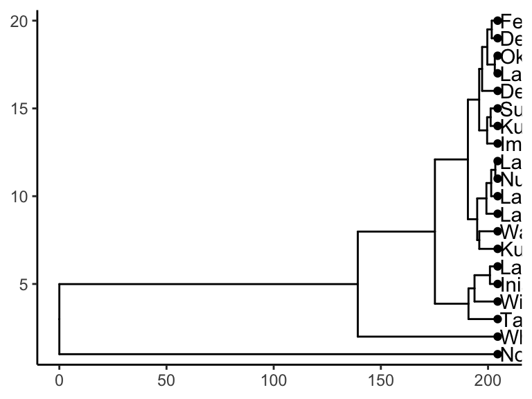
Cool! Though that plot could use some tweaking… let’s try:
AK_lakes_clustered %>%
ggtree() +
    geom_tiplab(aes(label = lake), offset = 10) +
    geom_tippoint(shape = 21, aes(fill = park), size = 4) +
    scale_x_continuous(limits = c(0,400))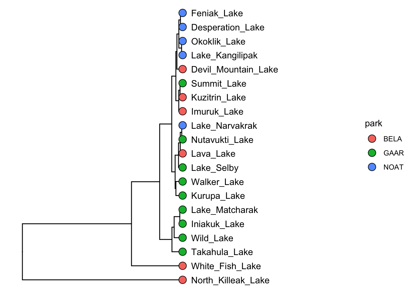
Very nice!
6.2 exercises
For this set of exercises, please use runMatrixAnalysis() to run and visualize a hierarchical cluster analysis with each of the main datasets that we have worked with so far, except for NY_trees. This means: algae_data (which algae strains are most similar to each other?), alaska_lake_data (which lakes are most similar to each other?). and solvents (which solvents are most similar to each other?). It also means you should use the periodic table (which elements are most similar to each other?), though please don’t use the whole periodic table, rather, use periodic_table_subset. For each of these, create (i) a tree diagram that shows how the “samples” in each data set are related to each other based on the numerical data associated with them, (ii) a caption for each diagram, and (iii) describe, in two or so sentences, an interesting trend you see in the diagram. You can ignore columns that contain categorical data, or you can list those columns as “additional_analyte_info”.
For this assignment, you may find the colnames() function and square bracket-subsetting useful. It will list all or a subset of the column names in a dataset for you. For example:
colnames(solvents)
##  [1] "solvent"             "formula"             "boiling_point"
##  [4] "melting_point"       "density"             "miscible_with_water"
##  [7] "solubility_in_water" "relative_polarity"   "vapor_pressure"
## [10] "CAS_number"          "formula_weight"      "refractive_index"
## [13] "specific_gravity"    "category"

colnames(solvents)[1:3]
## [1] "solvent"       "formula"       "boiling_point"

colnames(solvents)[c(1,5,7)]
## [1] "solvent"             "density"             "solubility_in_water"